While we wait to get a sense of Obama’s post-convention bounce, it’s worth taking a look at how predictive the trial-heat polls can be at this (or any) point of the campaign. I’ll use the state-level surveys from 2008 as a guide. Applying my model to these data, I can estimate the daily level of support for Obama vs. McCain in all 50 states, from May through November. We can then compare the candidates’ standing in the polls during the campaign to each state’s election outcome, and see how those differences varied over time.
To begin, here’s the trend in voter preferences in Florida in 2008. Polls are plotted as circles, for the percent supporting Obama (out of the total for Obama or McCain). The thick line is the model’s estimate of the underlying level of support for Obama. The horizontal line indicates the result of the election, in which Obama received 51.4% of the two-party vote.
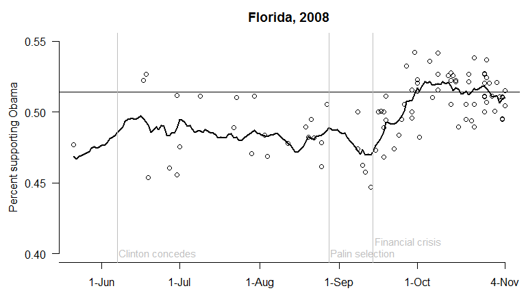
The trend is similar to what happened in most states: Obama polled behind his eventual vote share throughout the summer, then lost more ground following the RNC and selection of Sarah Palin. But once the the financial crisis began, Obama quickly gained in the polls – and by early October, the polls were about (on average) where the election ended up.
Next, I calculate the difference between each state’s daily estimate of voter opinion and the state’s election result, and average these across all 50 states. This is the mean absolute deviation, or MAD.
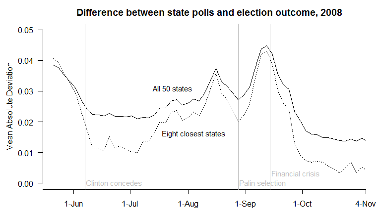
On average, the state polls (fed through my model) were off by 2%-3% through August, increasing to a maximum average error of 4% after the RNC. But by Election Day, the poll-based estimates only differed from the actual outcomes by an average of 1.4%. In states that were most competitive – and therefore polled more frequently – the error was even lower. If we isolate the eight closest states, where Obama finished with between 46% and 54% of the two-party vote, the average error on Election Day was a minuscule (and fairly remarkable) 0.4%.
So, in 2008, the polls were highly accurate over the last month of the campaign; and somewhat less so prior to that.
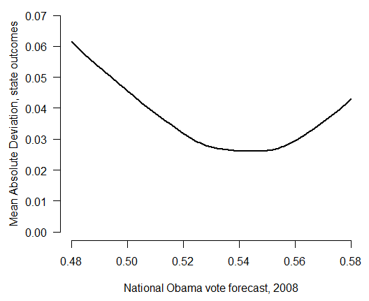
But looking at the polls isn’t the only way to predict the election outcome. In August and September of 2008, political scientists published a series of forecasts of the national-level vote, based upon long-term structural factors such as levels of economic growth, unemployment rates, whether the incumbent is running for re-election, and so forth. How well did these forecasts perform? The median prediction was that Obama would win 52% of the two-party vote. If we assume uniform swing and home-state effects relative to 2004 (as I describe here), this would have translated to an average state-level error of 3.2% – greater than that of the poll-based estimates for almost the entire campaign.
In fact, the minimum state-level MAD that any national-level election forecast could have produced in 2008 was 2.6%. Here I’ve plotted the state MAD under various assumptions about the national vote outcome (again, using uniform swing with home-state effects). The reason for this lower bound is that although uniform swing is an extremely useful model, it isn’t perfect. From election to election, state vote outcomes still tend to vary by an additional 3%-5% or more beyond the national swing.
The forecasts that I’m showing on this site are produced by combining long-term factors with estimates of current opinion based on the state polls. This stabilizes the forecasts relative to the polls alone, while also reducing the forecast MAD, as can be seen in my paper (Figure 4). In 2008, state forecasts using my model maintained an average error below 2% for the final two months of the campaign.
Leave a Reply