Evaluating the Forecasting Model

Since June, I’ve been updating the site with election forecasts and estimates of state-level voter preferences based on a statistical model that combines historical election data with the results of hundreds of state-level opinion polls. As described in the article that lays out my approach, the model worked very well when applied to data from the 2008 presidential election. It now appears to have replicated that success in 2012. The model accurately predicted Obama’s victory margin not only on Election Day – but months in advance of the election as well.

With the election results (mostly) tallied, it’s possible to do a detailed retrospective evaluation of the performance of my model over the course of the campaign. The aim is as much to see where the model went right as where it might have gone wrong. After all, the modeling approach is still fairly new. If some of its assumptions need to be adjusted, the time to figure that out is before the 2016 campaign begins.

To keep myself honest, I’ll follow the exact criteria for assessing the model that I laid out back in October.

1. Do the estimates of the state opinion trends make sense?

   Yes. The estimated trendlines in state-level voter preferences appear to pass through the center of the polling data, even in states with relatively few polls. This suggests that the hierarchical design of the model, which borrows information from the polls across states, worked as intended.

   The residuals of the fitted model (that is, the difference between estimates of the “true” level of support for Obama/Romney in a state and the observed poll results) are also consistent with a pattern of random sampling variation plus minor house effects. In the end, 96% of polls fell within the theoretical 95% margin of error; 93% were within the 90% MOE; and 57% were within the 50% MOE.

2. How close were the state-level vote forecasts to the actual outcomes, over the course of the campaign?

   The forecasts were very close to the truth, even in June. I calculate the mean absolute deviation (MAD) between the state vote forecasts and the election outcomes, on each day of the campaign. In the earliest forecasts, the average error was already as low as 2.2%, and gradually declined to 1.7% by Election Day. (Perfect predictions would produce a MAD of zero.)

   

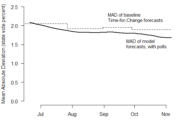
   By incorporating state-level polls, the model was able to improve upon the baseline forecasts generated by the Abramowitz Time-for-Change model and uniform swing – but by much less than it did in 2008. The MAD of the state-level forecasts based on the Time-for-Change model alone – with no polling factored in at all – is indicated by the dashed line in the figure. It varied a bit over time, as updated Q2 GDP data became available.

   Why didn’t all the subsequent polling make much difference? The first reason is that the Time-for-Change forecast was already highly accurate: it predicted that Obama would win 52.2% of the major party vote; he actually received 51.4%. The successful track record of this model is the main reason I selected it in the first place. Secondly, state-level vote swings between 2008 and 2012 were very close to uniform. This again left the forecasts with little room for further refinement.

   But in addition to this, voters’ preferences for Obama or Romney were extremely stable this campaign year. From May to November, opinions in the states varied by no more than 2% to 3%, compared to swings of 5% to 10% in 2008. In fact, by Election Day, estimates of state-level voter preferences weren’t much different from where they started on May 1. My forecasting model is designed to be robust to small, short-term changes in opinion, and these shifts were simply not large enough to alter the model’s predictions about the ultimate outcome. Had the model reacted more strongly to changes in the polls – as following the first presidential debate, for example – it would have given the mistaken impression that Obama’s chances of reelection were falling, when in fact they were just as high as ever.

3. What proportion of state winners were correctly predicted?

   As a result of the accuracy of the prior and the relative stability of voter preferences, the model correctly picked the winner of nearly every state for the entire campaign. The only mistake arose during Obama’s rise in support in September, which briefly moved North Carolina into his column. After the first presidential debate, the model returned to its previous prediction that Romney would win North Carolina. On Election Day, the model went 50-for-50.

4. Were the competitive states identified early and accurately?

   Yes. Let’s define competitive states as those in which the winner is projected to receive under 53% of the two-party vote. On June 23, the model identified twelve such states: Arizona, Colorado, Florida, Indiana, Iowa, Michigan, Missouri, Nevada, North Carolina, Ohio, Virginia, and Wisconsin. That’s a good list.

5. Do 90% of the actual state vote outcomes fall within the 90% posterior credible intervals of the state vote forecasts?

   This question addresses whether there was a proper amount of uncertainty in the forecasts, at various points in the campaign. As I noted before, in 2008, the forecasts demonstrated a small degree of overconfidence towards the end of the campaign. The results from the 2012 election show the same tendency. Over the summer, the forecasts were actually a bit underconfident, with 95%-100% of states’ estimated 90% posterior intervals containing the true outcome. But by late October, the model produced coverage rates of just 70% for the nominal 90% posterior intervals.

   As in 2008, the culprit for this problem was the limited number of polls in non-competitive states. The forecasts were not overconfident in the key battleground states where many polls were available, as can be seen in the forecast detail. It was only in states with very few polls – and especially where those polls were systematically in error, as in Hawaii or Tennessee – that the model became misled. A simple remedy would be to conduct more polls in non-competitive states, but it’s not realistic to expect this to happen. Fortunately, overconfidence in non-competitive states does not adversely impact the overall electoral vote forecast. Nevertheless, this remains an area for future development and improvement in my model.

   It’s also worth noting that early in the campaign, when the amount of uncertainty in the state-level forecasts was too high, the model was still estimating a greater than 95% chance that Obama would be reelected. In other words, aggregating a series of underconfident state-level forecasts produced a highly confident national-level forecast.

6. How accurate was the overall electoral vote forecast?

   The final electoral vote was Obama 332, Romney 206, with Obama winning all of his 2008 states, minus Indiana and North Carolina. My model first predicted this outcome on June 23, and then remained almost completely stable through Election Day. The accuracy of my early forecast, and its steadiness despite short-term changes in public opinion, is possibly the model’s most significant accomplishment.

   In contrast, the electoral vote forecasts produced by Nate Silver at FiveThirtyEight hovered around 300 through August, peaked at 320 before the first presidential debate, then cratered to 283 before finishing at 313. The electoral vote estimator of Sam Wang at the Princeton Election Consortium demonstrated even more extreme ups and downs in response to the polls.

7. Was there an appropriate amount of uncertainty in the electoral vote forecasts?

   This is difficult to judge. On one hand, since many of the state-level forecasts were overconfident, it would be reasonable to conclude that the electoral vote forecasts were overconfident as well. On the other hand, the actual outcome – 332 electoral votes for Obama – fell within the model’s 95% posterior credible interval at every single point of the campaign.

8. Finally, how sensitive were the forecasts to the choice of structural prior?

   Given the overall solid performance of the model – and that testing out different priors would be extremely computationally demanding – I’m going to set this question aside for now. Suffice to say, Florida, North Carolina, and Virginia were the only three states in which the forecasts were close enough to 50-50 that the prior specification would have made much difference. And even if Obama had lost Florida and Virginia, he still would have won the election. So this isn’t something that I see as an immediate concern, but I do plan on looking into it before 2016.