The site provides two different types of information. First, it estimates the trend in public opinion for Obama vs. Romney in each state up to the current day. But it also forecasts ahead to Election Day – given what we know now, what is the election outcome most likely to be? These forecasts are produced at both the state and national level, and are accompanied by a statement of uncertainty in each projection.
All of the estimates are based on a single, unified statistical model. The forecasting component combines data from past presidential elections with results from the large number of state-level opinion surveys released during the 2012 campaign. As new polls become available, the forecasts update in real time, gradually increasing in both accuracy and precision as Election Day nears.
The model is specifically designed to overcome the data limitation that not every state is polled on every day of the campaign. To smooth out and fill in any gaps in the polls, the model looks for common trends in voter preferences across states. These are usually the result of major campaign or news events that affect voters in all states at the same time. By drawing upon these patterns, the model is able to keep the election forecasts completely up-to-date.
The model is described in greater detail in a research article, Dynamic Bayesian Forecasting of Presidential Elections in the States, in the Journal of the American Statistical Association. Here’s the method I follow for this site.
The historical forecast
The first step is to generate a baseline structural forecast of each state’s election outcome from predictive long-term historical factors. I base my structural forecast on the Abramowitz Time-for-Change model, which has had an excellent track record.
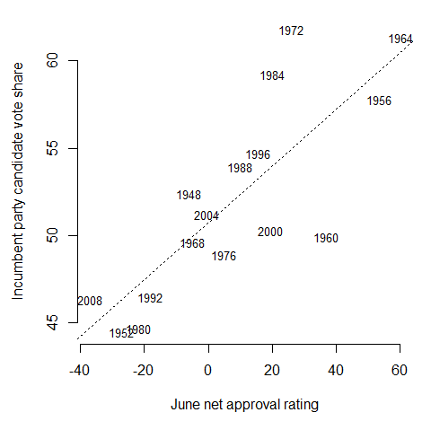
The Time-for-Change model predicts the incumbent party candidate’s national-level vote share as a function of three variables: the president’s net approval-disapproval rating in June of the election year; the percent change in GDP from Q1 to Q2 of the election year; and whether the incumbent party has held the presidency for two or more terms. For now, the 2012 Q2 GDP data aren’t available yet, so I use the change in GDP from the last quarter of 2011 to the first quarter of 2012 instead. The first official estimate of Q2 GDP growth – 1.5% – was released on July 27. The updated second estimate of Q2 GDP growth – 1.7% – was released August 29. The third estimate of Q2 GDP growth – 1.3% – was released September 27. Presidential approval data are from the Gallup survey organization, and economic data are from the U.S. Department of Commerce Bureau of Economic Analysis.
The June net approval rating is an especially useful measure. Going back to 1948, presidents that are more popular in June have been much more likely to get reelected in November.
The rest of the data are in the table below. The dependent variable is the incumbent party candidate’s share of the major-party vote.
| Incumbent | Incumbent | Incumbent | |||
| Q1 GDP | Q2 GDP | net approval | party 2+ | party cand. | |
| Year | growth | growth | rating, June | terms? | vote share |
| 2012 | 2.0 | 1.3 | -0.8 | 0 | — |
| 2008 | -1.8 | 1.3 | -37.0 | 1 | 46.3 |
| 2004 | 2.7 | 2.6 | -0.5 | 0 | 51.2 |
| 2000 | 1.1 | 8.0 | 19.5 | 1 | 50.3 |
| 1996 | 2.8 | 7.1 | 15.5 | 0 | 54.7 |
| 1992 | 4.5 | 4.3 | -18.0 | 1 | 46.5 |
| 1988 | 2.1 | 5.2 | 10.0 | 1 | 53.9 |
| 1984 | 8.0 | 7.1 | 20.0 | 0 | 59.2 |
| 1980 | 1.3 | -7.9 | -21.7 | 0 | 44.7 |
| 1976 | 9.4 | 3.0 | 5.0 | 1 | 48.9 |
| 1972 | 7.3 | 9.8 | 26.0 | 0 | 61.8 |
| 1968 | 8.5 | 7.0 | -5.0 | 1 | 49.6 |
| 1964 | 9.3 | 4.7 | 60.3 | 0 | 61.3 |
| 1960 | 9.3 | -1.9 | 37.0 | 1 | 49.9 |
| 1956 | -1.8 | 3.2 | 53.5 | 0 | 57.8 |
| 1952 | 4.1 | 0.4 | -27.0 | 1 | 44.5 |
| 1948 | 6.5 | 7.5 | -6.0 | 1 | 52.4 |
A multiple linear regression model fitted to the 16 elections from 1948-2008 indicates that
Incumbent vote share = 51.5 + 0.6 (Q2 growth) + 0.1 (Net approval) – 4.3 (Two+ terms).
Plugging in values from 2012, we’d expect Obama to receive about 52.2% of the two-party national vote. It’s worth noting that this is already a strong position.
To translate this to the state level, I exploit a pattern known as uniform swing. Since the 1980 presidential election, support for each party has tended to rise and fall in national waves, by similar amounts across states. Obama received 53.7% of the two-party national vote in 2008. So, I subtract the difference, 1.3%, from each of Obama’s 2008 state-level vote shares. Finally, I correct for home-state effects by subtracting 6% in Massachusetts for Romney and adding back 6% in Arizona for McCain.
Updating from pre-election polls
The state-level structural forecasts are used to specify an informative Bayesian prior over the outcome in each state. Until new polls are released, these forecasts represent our best guesses about what will happen on Election Day. Nevertheless, the baseline projections will contain errors. Since the aim is to get the forecasts right as soon as possible, state-level survey data are used to refine the baseline forecasts. As the campaign progresses, the model’s forecasts become based less on the historical data, and more on the current polls.
On any day of the campaign, the past trends and future forecasts of voter preferences in every state are estimated simultaneously, using whatever polls are currently available. I fit the model using a Bayesian MCMC sampling procedure that provides posterior uncertainty estimates which enable logically valid, probabilistic inferences about the election outcome. The error bars in the forecast detail and forecast tracker pages are all 95% credible intervals. For more on the model equations and other technical details, they’re in the article.
To do the updating, the model makes a series of assumptions; some for simplification, others to capture what we (think we) know about the dynamics of public opinion during a presidential election campaign. First, I translate every poll result into the proportion favoring Obama or Romney among only those respondents with a preference for either candidate. This sets aside anyone who is undecided – and is why all the survey results on the poll tracker page appear symmetrical. I consider this safer than making guesses about how those voters will ultimately decide on Election Day.
Next, I assume that the proportion supporting Obama in any given poll can be treated as if it were taken from a simple random sample (as most pollsters aspire to). I don’t attempt to “correct” in any way for other sources of survey error, house effects, weighting schemes, etc. My expectation is that with enough polling data, the various pollster biases will all cancel out. Usually this assumption is pretty safe. It’s most problematic in states that aren’t polled frequently – but fortunately, those states tend to be the least competitive, so mistakes there are less consequential.
The model then assumes that the proportion of voters supporting Obama in each state on a given day can be broken up into a state component – unique to each state – and a national component – shared by all states. The national component detects common trends in the polls, and enables the state opinion trends to be linked together over time; especially when polling data are scarce. The trend lines in the poll tracker section result from re-combining these two elements.
Finally, the model makes an assumption about the nature of the daily changes in the underlying state and national trends. It is simply that today’s best estimate for each series is equal to a small deviation – given the polls – from tomorrow’s best estimate. How do we know what tomorrow’s estimate will be? This is where the informative prior over the structural forecast comes back in. In a sense, the model works backwards from the expected outcome to the most recent polling data – and forwards from past polling data to connect at the current day.
Putting this all together, the Election Day forecast in each state is a compromise between the newest poll results and the predictions of the structural model. If a state’s baseline forecast is out of line with recent polling, it is automatically adjusted to align more closely with the polls. As older polls are superseded by newer information, they contribute less to the forecast, but they leave behind the estimated trend in opinion up to the current day of the campaign.
The data handling and graphics are all done in R. The estimation is performed using WinBUGS. Polling data are obtained from a variety of public sources, most helpfully the TPM Polltracker and HuffPost Pollster, aided by their Pollster API.
After the model is fitted, I calculate the probability that Obama or Romney will win each state directly from the posterior distribution of the Election Day forecasts. I then simulate the distribution of electoral votes each candidate is expected to receive, given these state forecasts. The site banner shows the trends in forecasts of the median electoral vote.
Does it work?
I validated the model with state-level pre-election polls from the 2008 presidential campaign, using the benefit of hindsight to evaluate model performance. In a simulated run-through of the campaign from May to November, the model was able to steadily improve the accuracy of its forecasts, ultimately mispredicting the winner of only a single state. By Election Day, the average difference between the model forecasts and the actual state election outcomes was just 1.4%, with more than half of states projected to within 1%. The model also correctly identified the competitive swing states very early in the campaign.
A second concern is whether the uncertainty in the state election forecasts is properly calibrated. In my simulation, I checked whether the 90% posterior credible intervals around each forecast actually included the true election outcome in 90% of states. I found the coverage rate to be correct until the final month of the campaign, when it dipped below 80%. However, this was primarily a function of limitations and anomalies in the underlying survey data, rather than significant flaws in the model. Most of the erroneous intervals were in states where very few polls had been conducted, so that a small number of inaccurate surveys had undue influence on the forecast. That said, because states that are polled infrequently also tend to be uncompetitive, there was very little practical consequence to the narrower than expected forecast intervals in these states.
Finally, I performed a sensitivity analysis on both the choice of structural forecasts, and the amount of prior confidence placed in them. Instead of the Time-for-Change model, I tried an inaccurate baseline calculated as the average Democratic vote share in the last four presidential elections in each state. Even from this starting point, the model updated the forecasts properly, and quickly identified Obama as the eventual winner. Slightly weakening the priors on the forecast did not have much of an effect on forecast accuracy or coverage rates. However, overly strong priors did generate misleadingly narrow posterior credible intervals. The priors I use for the analysis on this site are based on the calibration I conducted using the 2008 polls.