Polling Analysis and Election Forecasting

Category: Uncategorized (Page 2 of 7)

Forecasting the 2016 Elections

Welcome to Votamatic for the 2016 presidential election campaign.

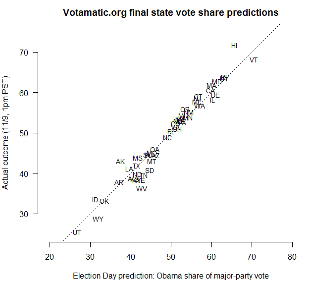
For those new to the site, I originally launched Votamatic in 2012 to track and forecast the presidential election between Barack Obama and Mitt Romney, based on some academic research I had been doing at the time. My early prediction of a 332-206 Obama win, using a combination of historical data, state-level public opinion polls, and a Bayesian statistical model turned out to be exactly correct. All of the data and results from 2012 have been archived, and can be reached from the top navigation bar.

The 2016 version of Votamatic is going to be fairly scaled back compared to 2012. I’ll still have poll tracking charts and the occasional blog post, but my election forecasts will be built into a brand new site at Daily Kos Elections that I’ve been helping to create. In 2014, I worked with the Daily Kos Elections team to forecast the midterm Senate and gubernatorial elections, with continued success. This year, we’re expanding the collaboration.

Over the next few weeks, we’ll be rolling out a bunch of new features, so stay tuned. Starting with presidential forecasts, we’ll soon add forecasts of every Senate and gubernatorial race in the nation (including the chances that the Democrats will retake the Senate), and sophisticated poll tracking charts and trendlines, all built on top of a custom polling database. The site will also feature Daily Kos Elections’ regular campaign reporting and analysis, as well as candidate endorsements and opportunities for getting involved. I hope you’ll find the site interesting, immersive, and accurate — and worth returning to as the campaign evolves.

(Sneak preview: Other election forecasters are giving Hillary Clinton around an 80-85% chance of winning. My interpretation of the polling data and other historical factors makes me a little less confident in a Clinton victory, but not much so; I’ll have more to say on this soon. Either way, the election is still far from a done deal. Flip a coin twice: if you get two heads, that’s President Trump.)

I will update the trendlines on this site every day or two, as new polls come in. Every state that has at least one poll will get a trendline. To see the polling data and trends together, go to the Poll Tracker page. For a zoomed-in view of each state’s trendline, check out the State Trend Detail pages.

The statistical model that I use to produce these trendlines has a set of features that are designed to reveal, as clearly as possible, the underlying voter preferences in each state during the campaign. Looking at the poll tracker in Florida, for example, Clinton (blue) led until mid-July, when she was overtaken by Trump (red). After the Democratic National Convention, however, Clinton’s numbers rebounded to move her back into a slight lead.

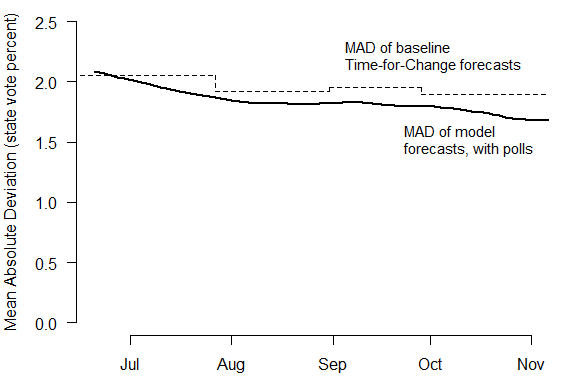
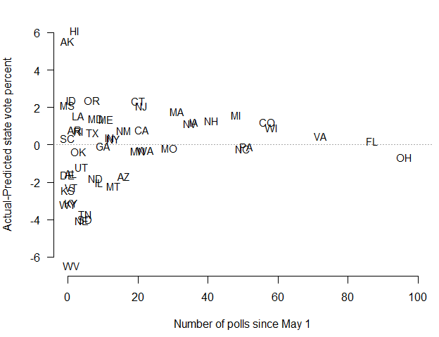
States with more polls will have more accurate trendline estimates. But my model produces a complete trendline for each candidate in any state that has at least one poll. To do this, it looks for common patterns in public opinion across multiple states over time, and uses those to infer a national trend. (This works because changes in voter preferences are largely — though certainly not entirely — a response to national-level campaign effects.) The model then applies those trends back into each state, adjusting for each state’s unique polling data. States in which no polls have been conducted are displayed as empty plots, awaiting more data.

The trendlines that you will see here track Clinton and Trump in a head-to-head matchup only, excluding third-party candidates and voters who say they are undecided. This has the benefit of removing idiosyncrasies from the polling data around question wording, survey methodology, whether a pollster “pushes” respondents who are leaning towards either candidate into making a decision, and so forth. Visually, this explains why the trendlines for Clinton and Trump are mirror images of each other: the Clinton and Trump percents have been rescaled to sum to 100%. On the other hand, this sacrifices a lot of potentially interesting information about each race. The trendlines we’ll have at Daily Kos Elections will include other candidates and undecideds.

Finally, I account for two other features of each poll. Polls with larger sample sizes are given more weight in fitting the trendlines, relative to polls with smaller sample sizes. And if a poll was conducted by a partisan polling firm, the model subtracts 1.5% from the reported vote share of the candidate from the respective party. So, for example, if a Democratic pollster reports a race tied at 50%-50%, the model treats the poll as showing a three point Trump lead, 51.5%-48.5%. Those are the only adjustments I make to the raw polling data, assuming that all other survey errors will cancel each other out as noise.

See you soon, over at Daily Kos Elections!

2014 Senate and Governor Forecasts

This election season, I’ve been doing some work with the Daily Kos Elections team to track and forecast the midterm Senate and Gubernatorial elections. To see our predictions, click over to the Senate Outlook and Governors Outlook. You can also read more about our modeling approach here.

Overall, the polls aren’t looking good for Senate Democrats this year. We predict a 90% chance that Republicans will gain control of the Senate (assuming the public polls can be trusted). The most likely outcome is a 53-seat Republican majority. On the Gubernatorial side, the situation is better for the Democrats, but there are still a lot of close races — and a lot of uncertainty. It’s possible that Democrats could end up controlling anywhere from 16 to 27 states; they currently control 21.

For Election Night resources, I can recommend:

For more on the similarities and differences between the major midterm election forecasting models, Vox and the Washington Post both had very nice overviews of how Senate forecasts are typically made, how they should be interpreted, and how to judge their predictions after the election.

Evaluating the Forecasting Model

Since June, I’ve been updating the site with election forecasts and estimates of state-level voter preferences based on a statistical model that combines historical election data with the results of hundreds of state-level opinion polls. As described in the article that lays out my approach, the model worked very well when applied to data from the 2008 presidential election. It now appears to have replicated that success in 2012. The model accurately predicted Obama’s victory margin not only on Election Day – but months in advance of the election as well.

With the election results (mostly) tallied, it’s possible to do a detailed retrospective evaluation of the performance of my model over the course of the campaign. The aim is as much to see where the model went right as where it might have gone wrong. After all, the modeling approach is still fairly new. If some of its assumptions need to be adjusted, the time to figure that out is before the 2016 campaign begins.

To keep myself honest, I’ll follow the exact criteria for assessing the model that I laid out back in October.

  1. Do the estimates of the state opinion trends make sense?

    Yes. The estimated trendlines in state-level voter preferences appear to pass through the center of the polling data, even in states with relatively few polls. This suggests that the hierarchical design of the model, which borrows information from the polls across states, worked as intended.

    The residuals of the fitted model (that is, the difference between estimates of the “true” level of support for Obama/Romney in a state and the observed poll results) are also consistent with a pattern of random sampling variation plus minor house effects. In the end, 96% of polls fell within the theoretical 95% margin of error; 93% were within the 90% MOE; and 57% were within the 50% MOE.

  2. How close were the state-level vote forecasts to the actual outcomes, over the course of the campaign?

    The forecasts were very close to the truth, even in June. I calculate the mean absolute deviation (MAD) between the state vote forecasts and the election outcomes, on each day of the campaign. In the earliest forecasts, the average error was already as low as 2.2%, and gradually declined to 1.7% by Election Day. (Perfect predictions would produce a MAD of zero.)

    By incorporating state-level polls, the model was able to improve upon the baseline forecasts generated by the Abramowitz Time-for-Change model and uniform swing – but by much less than it did in 2008. The MAD of the state-level forecasts based on the Time-for-Change model alone – with no polling factored in at all – is indicated by the dashed line in the figure. It varied a bit over time, as updated Q2 GDP data became available.

    Why didn’t all the subsequent polling make much difference? The first reason is that the Time-for-Change forecast was already highly accurate: it predicted that Obama would win 52.2% of the major party vote; he actually received 51.4%. The successful track record of this model is the main reason I selected it in the first place. Secondly, state-level vote swings between 2008 and 2012 were very close to uniform. This again left the forecasts with little room for further refinement.

    But in addition to this, voters’ preferences for Obama or Romney were extremely stable this campaign year. From May to November, opinions in the states varied by no more than 2% to 3%, compared to swings of 5% to 10% in 2008. In fact, by Election Day, estimates of state-level voter preferences weren’t much different from where they started on May 1. My forecasting model is designed to be robust to small, short-term changes in opinion, and these shifts were simply not large enough to alter the model’s predictions about the ultimate outcome. Had the model reacted more strongly to changes in the polls – as following the first presidential debate, for example – it would have given the mistaken impression that Obama’s chances of reelection were falling, when in fact they were just as high as ever.

  3. What proportion of state winners were correctly predicted?

    As a result of the accuracy of the prior and the relative stability of voter preferences, the model correctly picked the winner of nearly every state for the entire campaign. The only mistake arose during Obama’s rise in support in September, which briefly moved North Carolina into his column. After the first presidential debate, the model returned to its previous prediction that Romney would win North Carolina. On Election Day, the model went 50-for-50.

  4. Were the competitive states identified early and accurately?

    Yes. Let’s define competitive states as those in which the winner is projected to receive under 53% of the two-party vote. On June 23, the model identified twelve such states: Arizona, Colorado, Florida, Indiana, Iowa, Michigan, Missouri, Nevada, North Carolina, Ohio, Virginia, and Wisconsin. That’s a good list.

  5. Do 90% of the actual state vote outcomes fall within the 90% posterior credible intervals of the state vote forecasts?

    This question addresses whether there was a proper amount of uncertainty in the forecasts, at various points in the campaign. As I noted before, in 2008, the forecasts demonstrated a small degree of overconfidence towards the end of the campaign. The results from the 2012 election show the same tendency. Over the summer, the forecasts were actually a bit underconfident, with 95%-100% of states’ estimated 90% posterior intervals containing the true outcome. But by late October, the model produced coverage rates of just 70% for the nominal 90% posterior intervals.

    As in 2008, the culprit for this problem was the limited number of polls in non-competitive states. The forecasts were not overconfident in the key battleground states where many polls were available, as can be seen in the forecast detail. It was only in states with very few polls – and especially where those polls were systematically in error, as in Hawaii or Tennessee – that the model became misled. A simple remedy would be to conduct more polls in non-competitive states, but it’s not realistic to expect this to happen. Fortunately, overconfidence in non-competitive states does not adversely impact the overall electoral vote forecast. Nevertheless, this remains an area for future development and improvement in my model.

    It’s also worth noting that early in the campaign, when the amount of uncertainty in the state-level forecasts was too high, the model was still estimating a greater than 95% chance that Obama would be reelected. In other words, aggregating a series of underconfident state-level forecasts produced a highly confident national-level forecast.

  6. How accurate was the overall electoral vote forecast?

    The final electoral vote was Obama 332, Romney 206, with Obama winning all of his 2008 states, minus Indiana and North Carolina. My model first predicted this outcome on June 23, and then remained almost completely stable through Election Day. The accuracy of my early forecast, and its steadiness despite short-term changes in public opinion, is possibly the model’s most significant accomplishment.

    In contrast, the electoral vote forecasts produced by Nate Silver at FiveThirtyEight hovered around 300 through August, peaked at 320 before the first presidential debate, then cratered to 283 before finishing at 313. The electoral vote estimator of Sam Wang at the Princeton Election Consortium demonstrated even more extreme ups and downs in response to the polls.

  7. Was there an appropriate amount of uncertainty in the electoral vote forecasts?

    This is difficult to judge. On one hand, since many of the state-level forecasts were overconfident, it would be reasonable to conclude that the electoral vote forecasts were overconfident as well. On the other hand, the actual outcome – 332 electoral votes for Obama – fell within the model’s 95% posterior credible interval at every single point of the campaign.

  8. Finally, how sensitive were the forecasts to the choice of structural prior?

    Given the overall solid performance of the model – and that testing out different priors would be extremely computationally demanding – I’m going to set this question aside for now. Suffice to say, Florida, North Carolina, and Virginia were the only three states in which the forecasts were close enough to 50-50 that the prior specification would have made much difference. And even if Obama had lost Florida and Virginia, he still would have won the election. So this isn’t something that I see as an immediate concern, but I do plan on looking into it before 2016.

Final Result: Obama 332, Romney 206

The results are in: Obama wins all of his 2008 states, minus Indiana and North Carolina, for 332 electoral votes. This is exactly as I predicted on Tuesday morning – and as I’ve been predicting (albeit with greater uncertainty) since June. Not bad! The Atlantic Wire awarded me a Gold Star for being one of “The Most Correct Pundits In All the Land”. There were also nice write-ups in The Chronicle of Higher Education, BBC News Magazine, Atlanta Journal-Constitution and the LA Times, among others. Thanks to everyone who has visited the site, participated in the comments, and offered their congratulations. I really appreciate it.

I’m still planning a complete assessment of the performance of the forecasting model, along the lines I described a few weeks ago. But in the meantime, a few quick looks at how my Election Day predictions stacked up against the actual state-level vote outcomes. First, a simple scatterplot of my final predictions versus each state’s election result. Perfect predictions will fall along the 45-degree line. If a state is above the 45-degree line, then Obama performed better than expected; otherwise he fared worse.

Interestingly, in most of the battleground states, Obama did indeed outperform the polls; suggesting that a subset of the surveys in those states were tilted in Romney’s favor, just as I’d suspected. Across all 50 states, however, the polls were extremely accurate. The average difference between the actual state vote outcomes and the final predictions of my model was a miniscule 0.03% towards Obama.

My final estimates predicted 19 states within 1% of the truth, with a mean absolute deviation of 1.7%, and a state-level RMSE of 2.3% (these may change slightly as more votes are counted). Other analysts at the CFAR blog and Margin of Error compared my estimates to those of Nate Silver, Sam Wang, Simon Jackman, and Josh Putnam, and found they did very well. All in all, a nice round of success for us “quants”.

Unsurprisingly, my model made much better predictions where more polls had been fielded! Here I’ll plot the difference between Obama’s share of the two-party vote in each state, and my final prediction, as a function of the number of polls in the state since May 1. Again, positive values indicate states where Obama did better than expected.

For minimizing the error in my forecasts, the magic number of polls per state appears to be around 25. That’s really not a lot; and I’m hopeful that we can get to at least this number in 2016. It’s a bit concerning, though, that there were about 25% fewer state-level presidential polls this year, compared to 2008.

Recently there have been some complaints among pollsters – most notably Gallup’s Frank Newport – that survey aggregators (like me) “don’t exist without people who are out there actually doing polls,” and that our work threatens to dissuade survey organizations from gathering these data in the first place. My view is slightly different. I’d say that working together, we’ve proven once again that public opinion research is a valuable source of information for understanding campaign dynamics and predicting election outcomes. There’s no reason why the relationship shouldn’t be one of mutual benefit, rather than competition or rivalry. In a similar manner, our analyses supplement – not replace – more traditional forms of campaign reporting. We should all be seen as moving political expertise forward, in an empirical and evidence-based way.

Election Day Forecast: Obama 332, Romney 206

With the last set of polls factored into the model, my final prediction is Obama to win 332 electoral votes, with 206 for Romney. This is both the median and the modal outcome in my electoral vote simulation, and corresponds to Obama winning all of his 2008 states except Indiana and North Carolina.

The four closest states – and therefore the most difficult to predict – are Florida, North Carolina, Virginia, and Colorado. Of these, my model only expects Romney to win North Carolina; but Florida is a true toss-up, with just a 60% chance of Obama victory. I would not be surprised if Florida ended up going for Romney. If that happens, Obama would win 303 electoral votes, which is the second-most likely scenario in my simulation. The third-most likely scenario is that Obama wins 347 electoral votes, picking up North Carolina in addition to Florida.

It’s been interesting to watch the forecasts of other poll watchers converge on the 332 estimate. Sam Wang, at the Princeton Election Consortium, also sees 332 as the modal outcome. So does Simon Jackman at the Huffington Post, and Josh Putnam at FHQ. Nate Silver, at his FiveThirtyEight blog, reports the mean of his electoral vote simulation at 313 – effectively splitting the difference on Florida, which he currently rates a 50.3% chance of an Obama win. But his most likely outcome is still Obama 332, followed by 303 and 347, just like me. Update: both Wang and Jackman revised their forecasts slightly downward this afternoon, based on late-arriving polls.

There will be plenty of opportunities to evaluate all of these forecasts once the election results are known. I’ve already laid out the standards I’ll be using to check my own model. This is how quantitative election forecasting can make progress, and hopefully work even better next time.

I’ll add, though, that on the eve of the election, averaging the polls, or running them through any sort of sensible model, isn’t all that hard. We are all using the same data (more or less) and so it doesn’t surprise me that we’re all reaching similar conclusions. The real challenge is producing meaningful and accurate forecasts early in the campaign. My model is designed to be robust to short-term fluctuations in the polls, and converge in a stable and gradual manner to the final, Election Day estimates. It appears that in this regard, the model has worked as intended.

But from a broader perspective, my model has been predicting that Obama will win 332 electoral votes – give or take – since June. If all of us are correct today, the next question to ask is when each model arrived at the ultimate outcome. That’s a big if, though. Let’s start with how the votes come in tonight, and go from there.

« Older posts Newer posts »

© 2024 VOTAMATIC

Theme by Anders NorenUp ↑